The Fundamentals of Economics

A production possibilities curve (frontier) is a model that shows alternative ways that an entity can use its scarce resources. The model displays trade-offs, opportunity costs, scarcity, and efficiency.
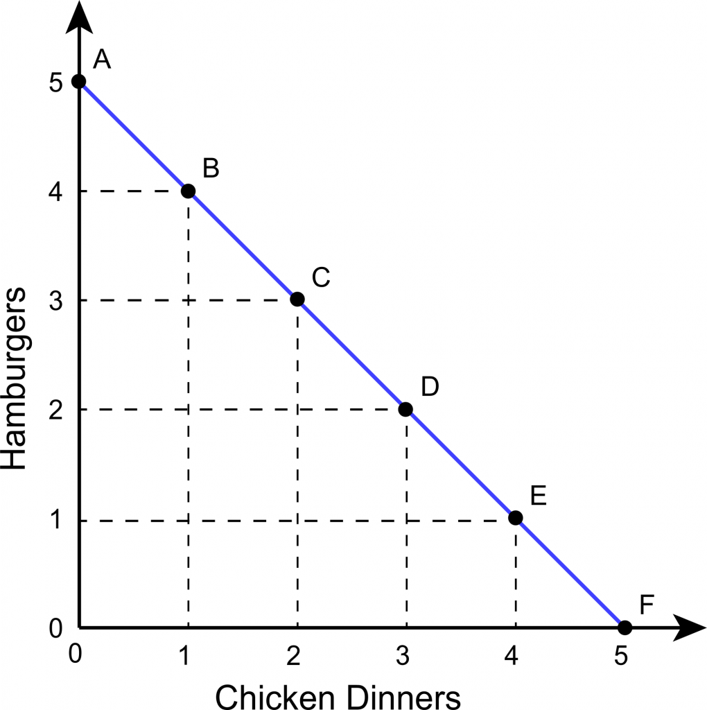
In the example below, a production possibilities curve (PPC) is used to chart the quantity of hamburgers and chicken dinners that can be made. If five hamburgers are made, zero chicken dinners are made, and so on.

	A	B	C	D	E	E
Hamburgers	5	4	3	2	1	0
Chicken Dinners	0	1	2	3	4	5

Points on a PPC can fall into three areas:

• Inside the curve – represents inefficiency/unemployment
• Outside the curve – are not possible with the given resources
• On the curve – represents efficiency

When points fall on the curve, all resources, like restaurant equipment and workers, are being used to produce the two items. There is a constant opportunity cost in this example, resulting in a straight line PPC. This means that the same adaptable resources are used for making both items. This is uncommon.

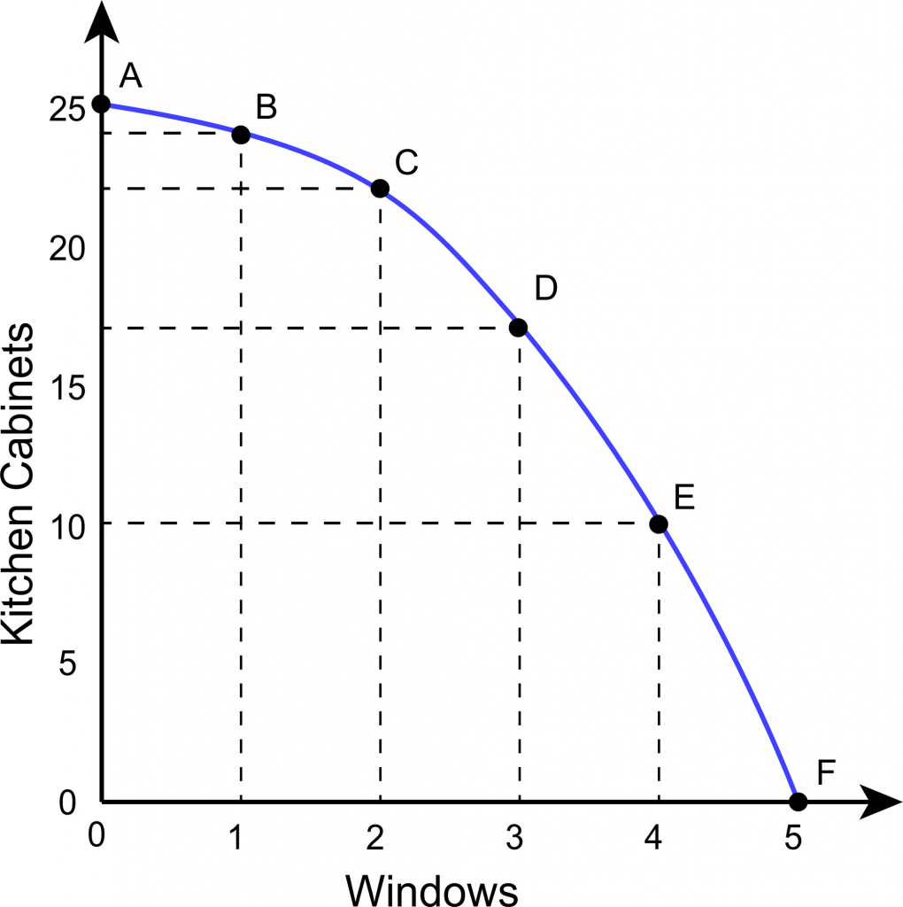
In contrast, the law of increasing opportunity cost states that as more of any item is produced, the opportunity cost (production of another item that was given up) increases. In other words, when two goods are produced, an increasing amount of the second good is given up. The reason is that resources are not easily adaptable between the production of the two items. In these cases, the PPC has a concave (inward) curve.

The information below can be charted with a concave curve. As more windows are made, fewer kitchen cabinets are made (opportunity cost increases).

	A	B	C	D	E	E
Kitchen Cabinets	25	24	22	17	10	0
Windows	0	1	2	3	4	5

Four key assumptions are made when analyzing production possibilities:

• Resources are used to produce one or both of only two goods.
• The amount of available resources does not change.
• Technology and production techniques do not change.
• Resources are used in a technically efficient way.